Piping fatigue and corrosion

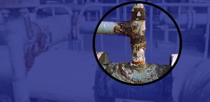
ASME B31.3 contains the footnote ‘Corrosion can sharply decrease cyclic life; therefore, corrosion resistant materials should be considered where a large number of major stress cycles is anticipated’. But what happens if carbon steel with high corrosion allowance has been selected and changes are out of the question? Or you may be assessing an existing system with heavy wall loss and many past cycles. In this article we’ll look at the usual ways to account for wall loss in fatigue calculation, and introduce a couple of alternative formulae.

Environmental correction factors

The ASME VIII Division 2 non-welded fatigue curve includes conservatism which is intended to address differences between real-world and laboratory test conditions. A factor of 4 on cycles is included to address both environmental and surface finish effects (see API 579 Table 14.8).

The British pressure vessel standard PD5500 states that it does not include any allowances for corrosive conditions, and recommends that a factor be chosen based on experience or testing.

British standard BS7608 downgrades un-welded components to account for the concentration effect of pitting, however this only brings it into alignment with the unwelded component curve given in PD5500. It also specifies a fatigue life reduction factor of 3 for freely corroding material in seawater.

US nuclear regulatory guide 1.207 provides correction factors to account for the effect of Light-Water Reactor environments.

It is not usually stated whether such factors account for loss of wall thickness as opposed to the localised effect of environment on stress concentration and crack growth. However, as the rate of wall loss is the same for any thickness, it is clear that factors don’t provide consistent adjustment for the reduction in section properties. Also, the same factor would apply whether the cycles occurred over 30 days or 30 years.

Therefore it is inferred that wall loss should be considered separately.

Varying wall thickness with time

Fatigue curves are based on a power relationship between stress range and number of cycles. Therefore, relatively small changes in stress range make quite a large difference to the result. If wall loss is expected to be significant for a new installation, or if it’s known to be significant for an existing system, how should this be catered for in analysis?

Lets assume we have a target lifetime for the system. You could simply subtract the maximum expected corrosion at end of life before calculating the stress range. This would give a very conservative estimate of fatigue life.

Another approach would be to construct a spreadsheet which breaks down the target life into steps of say 1 year each. You would subtract a proportion of the corrosion allowance each year, recalculate stress range and the corresponding allowable number of cycles. The damage for each year is then calculated and all years are summed by miner’s rule. This approach has advantages such as being able to consider different corrosion rates or thermal cycle ranges during the life of the system.

For a constant corrosion rate and thermal range, one would expect intuitively that subtracting half of the full corrosion is reasonable for a single representative calculation. So lets make a derivation of the ‘mathematically correct’ fatigue useage and then compare these approaches.

Fatigue useage formula

Fatigue curves typically take the form

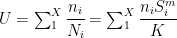
-where S is the range of equivalent stress between two states (eg. hot and cold). K is a factor accounting for the quality and type of welding, inspection, finishing and the degree of conservatism. The value of ‘m’ is typically taken as 3 for welded ferrous metals.

Using miner’s rule for Fatigue Useage (a.k.a. Damage) –

for continually varying stress range –

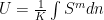
If the stress range is increasing lineally with cycles, from  to over cycles –

         -Eqn 1

The above is a reasonable and conservative approximation for moderate corrosion.

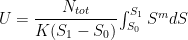
A more accurate relationship considers that the stress range is inversely proportional to thickness. For constant corrosion rate –

where c represents the total corrosion and t is thickness.

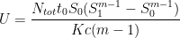
This can be used to derive an alternative equation for Useage. Lets skip the working this time and go straight to the final equation –

          -Eqn 2

Comparison of approaches

Typically, fatigue calculations which account for corrosion will assume the fully corroded condition, or perhaps half of the full corrosion. Let’s compare results for these and the other approaches shown here. We’ll use PD5500 fatigue curve F2 with no Young’s modulus correction, and consider both a low corrosion and a high corrosion case.

Results show that the ‘Average stress’ approach is pretty close to the ‘theoretically correct’ approach of Equation 2. Using the full corrosion allowance is much too conservative, while no corrosion is of course the opposite. Taking the average of the damage calculations for fully corroded and no corrosion is a little on the conservative side, as is Equation 1.

European and American fatigue curves

The European curves, such as those found in EN13445, DNV RP-C203 and PD5500 all follow the relationship shown here. The ASME VIII Division 2 welded fatigue curve follows this relationship as well, with ‘m’ equal to 3.13.

The ASME VIII non-welded fatigue curve does not follow the above relationship exactly, however by isolating the area of interest it can usually be fitted quite well to the formula. We just need to be careful to convert stress amplitude from the chart to stress range if using the formulae here. The stress amplitude must also be adjusted with a weld-related SCF where applicable, whereas the European standards provide different K-values for different weld types.

The B31 stress range reduction factor is also a form of fatigue curve, however it uses an ‘m’ value of 5. Therefore it is quite widely agreed that the B31 approach is not really accurate for high cycle fatigue in particular.

Aside – CAESAR II bug

There is a bug which I’ve noticed in CAESAR II for stress calculations at corroded intersections. Now it may have been corrected but it has been there for at least version 8 and below.

The option ‘all cases corroded’ is meant to remove corrosion from the wall thickness used for section modulus calculation. For reducing branches however, something is going wrong with the calculation. To test if your version of CAESAR II has this bug, simply enter a very high corrosion allowance for a reducing branch pipe, one that takes the wall thickness close to zero on the branch. With the ‘All cases corroded’ setting, the expansion or fatigue stress at the intersection should be sky-high – if not, then you’re seeing this bug.